Customer Choice Model and Attraction Effect

Context

Modeling customers' choices is a key technique in analyzing how purchase decisions are made and also, being able to quantify the magnitude of feature trade-offs across product functions in a customer's decision process.

The basic idea of a choice model is to analyze which product a customer would prefer to purchase when she is presented with a collection of choices. For example, in fashion we want to analyze the scale of preference toward buying a black Gucci wallet priced at $2000 vs other choices of designers/colors priced $1500 to $3000. Most of the time, we are interested in much larger choice combinations (e.g. materials, promotion, shape).

Traditional approaches to choice models (e.g. MLM) assumes IIA (Independence of Irrelevant Alternatives), which cannot represent certain key phenomena. Several non-parametric methods have been studied and proposed; as we explored many of them, 4 proposed an interesting RBM variation that extends MLM to represent several scenarios where choices vary among customers. It is also straightforward to implement. Here is our quick and simple experiment.

Problem Formulation

Our goal is to estimate individual the trade-off effect of purchase given a choice set. Eventually, we want to apply the individual trade-off effect to all customers who we can observe such behavior. Beyond trade-off, we are also interested in attraction effect – a driving force of a product to alternative products when it is presented in the choices.

Many types of source data coming to mind when approaching this problem. Among them, website behavior is by far the richest; also we can directly observe each visitor's choices and her final selection. For each visitor to the website, we construct her choice set from products she viewed; the final selection is the product she purchased. We consider this level of design as demand based choice model.

In our experiments, we explored other forms of problem designs, and each one of them reflects very different types of choice phenomena. For instance, we can treat a visitor’s purchases as our choice set, and then the select set represents only those products she eventually kept and not returned. This problem design reflects some subtle decision as related to actual fit, size, quality or price change. We called this problem design utility based choice model.

There are many such designs can be defined based on the business use cases. Here we share the experiment of demand based choices.

RBM Network

In our experiment the size of choice set is 18000 (total number of unique styles). The average choices (average number of unique styles per visitor) is around 13. We implemented the solution using Python + Chainer on three NVIDIA GeForce TITAN X GPUs. The network is a binary RBM (visible and hidden) with adaptive weight decay. To speed up the training, we adopt K-contrastive divergence learning, which performs adaptive K-steps Gibbs sampling. The weights are updated through reconstruction error on the visible layer via sigmoid cross entropy.a

Results

We used the trained hidden-to-visible weights to calculate choice rate, which is given by the formula:

$$\lambda(A|\mathcal{X}) = \displaystyle\sum_{h}exp(-E_{\theta}((\upsilon^{\mathcal{X}}, \omega^{A}), h)) = exp(b_{A})\displaystyle\prod_{k}\sum_{h_{k} \in \{0,1\}}exp((T_{\mathcal{X}}^k + U_{A}^k)h_{k})$$

We can use these probabilities to compare any two products in a choice set.

Example:

alt text

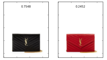
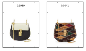
We can also use our validation data to contruct actual choice sets and compare those with network calculations.

Example:

Take the most frequent pairs of products in our validation data.
Calculate their choice rate (this will be the "theoretical").
Using validation data, calculate their choice rate from each choice set that they occur in (this will be the "actual").
Calculate the KL-Divergence between these two distributions and use this metric as the graph weight.

alt test

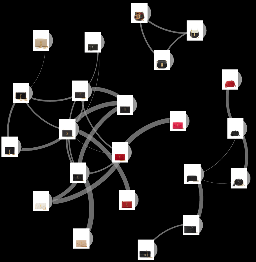
We can also calculate an attraction effect. If we have two products in a choice set, how does the addition of a third product affect customer choice? The strength of the attraction effect of a product C on A is defined as:

$$\psi_{A,C,\mathcal{X}}^{(att)}\equiv\frac{p(A|\mathcal{X} \cup \{C\})}{p(A|\mathcal{X})}$$

When this equation is greater than one there is an attraction effect.
Product B is preferred much more than product A.

alt text

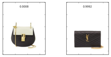
After the addition of a product C, the probability of product A has increased almost 15 fold.

alt text

$$\frac{0.011424}{0.000762} = 14.987$$

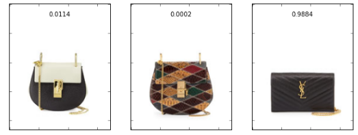
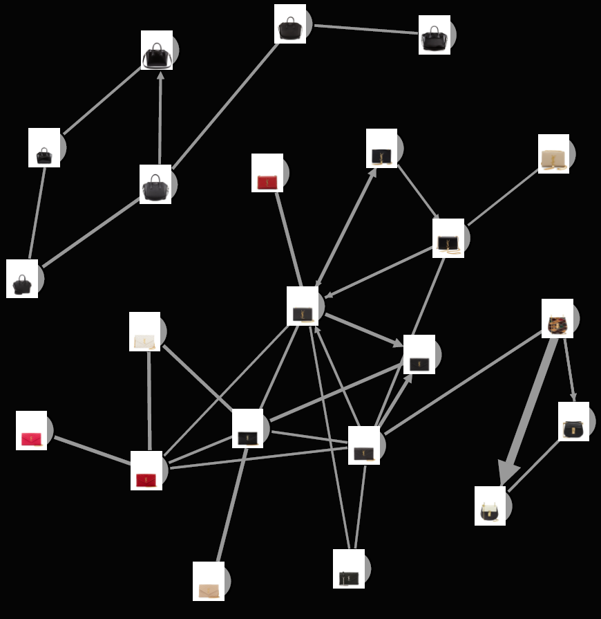
While not all product combinations exhibit this attractive behavior, several do and can be represented in a graph where the attractiveness is represented as an arrow (note our example in the bottom-right corner).

alt text